Basics

Details

Tutorials

Files

Oscill8 Tutorial #1: Chapter 10 Serious

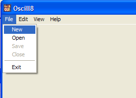
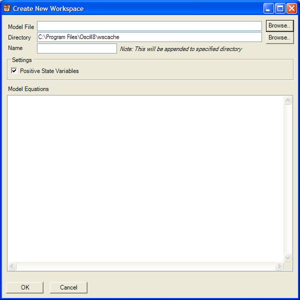
• Assuming you've installed Oscill8 correctly, we can start by opening Oscill8 (by double-clicking the icon on your desktop or by finding it under the Start Menu --> All Programs --> Oscill8 menu) and navigating to File --> New. This will bring up the workspace creation dialog.

  
  

• Now, click Browse for the Model File and navigate to the Oscill8 install directory (most likely C:\Program Files\Oscill8). Go into the ode directory and select chap10_serious.ode. You should see the following: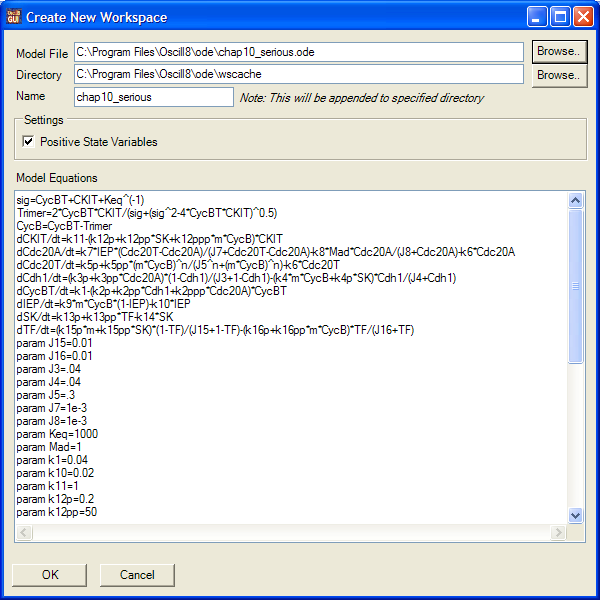

  

  You can select a different directory to place all the workspace files in, but by default that will be the same directory where the ODE file was with "wscache/<workspace_name>" appended to it. In some cases, you may choose to change certain settings, like "Positive State Variables" etc. In our case, just click OK to get started.

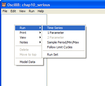
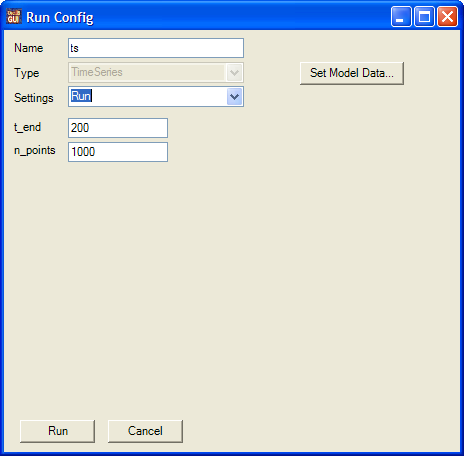
• There will be a momentary pause while Oscill8 interprets the model and creates the necessary files. The first order of business is to run a time series (solve the ODEs). In the run hierarchy area (the empty area to the left), alt-click --> Run --> TimeSeries. This will bring up the run configuration window.

  
  

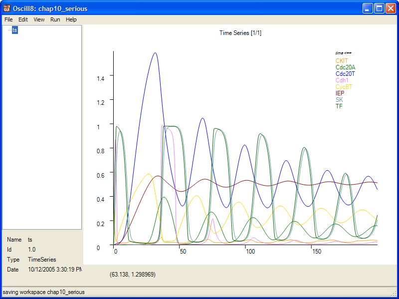
• Change t_end to 200 and n_points to 1000, then click Run; this will solve the ODEs for 200 time units and return 1000 data pionts along this solution.

  

• Now, there are a number of convenient key sequences to try to adjust the graphic properties. First, double-click inside the graphic portion of the window; then try x, y (adding shift reverses the sense of these arguments) to stretch (or squeeze, with shift) the x and y-axes, respectively. Try l to toggle the legend, try r to reset/refit the axes to the data, and then try clicking on the legend to toggle displayed data. Alt-clicking on the legend will bring up the line properties options, include curve color and width. For example, alt-click the yellow "CycBT"; change it's width to 5 and it's color to DarkOrange. Here's what you'll see (I've also clicked x once):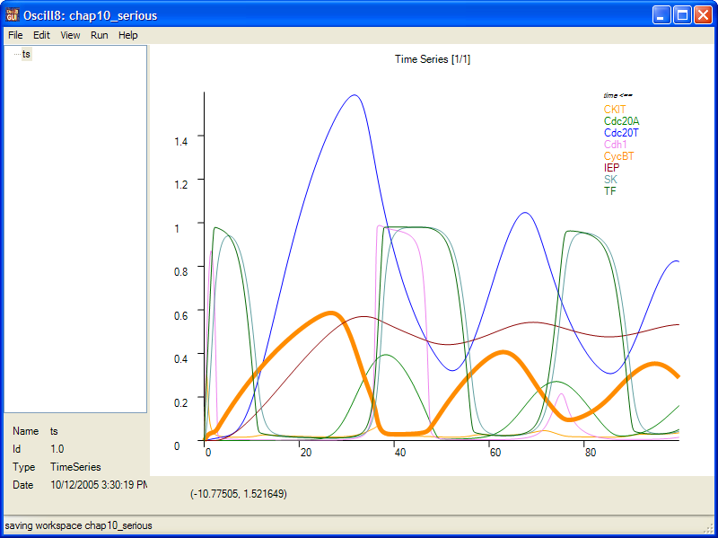

  

• There are also a bunch of options settable through the plot properties dialog, which you can get to by typing p, or by alt-clicking in the plot (not on the legend) and choosing "Plot Properties...".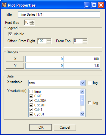

  

  Through the plot props dialog, you can move the position of the legend, toggle its visibility, manually set the x and y data ranges, and choose which variables are plotted against which variable (naturally, only one x variable may be plotted at a time, against any number of others). Just for fun, let's plot a phase plot of "CycBT" on the y-axis vs. "IEP" on the x-axis. This will produce (you'll need to click r to reset the plot to the data):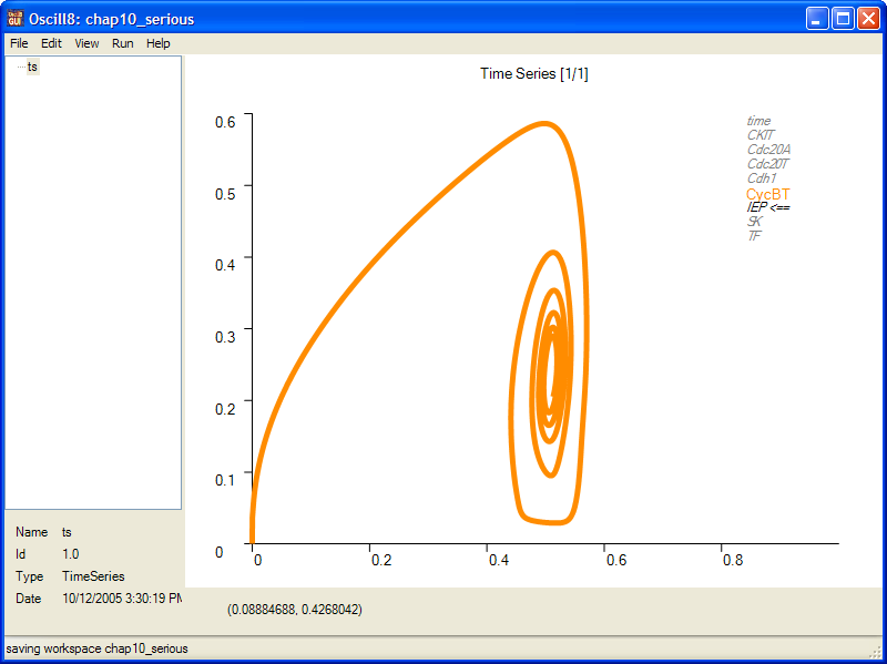

  

  It's important at this point to notice that in the legend, only the "CycBT" is highlighted and you'll see a <== next to the variable plotted on the x-axis.

• Now, let's get to the good stuff, bifurcation analysis! Oscill8 uses AUTO to do many one and two-parameter continuations of steady states and bifurcation curves. Alt-click in the history area and choose Run --> 1 Parameter. This gives you a run config dialog; scroll down the parameter list and double-click on the parameter m (you can, in fact, choose multiple--or all--parameters; in this case, the output is "scrolled" through in the output graphic using the up and down arrow keys):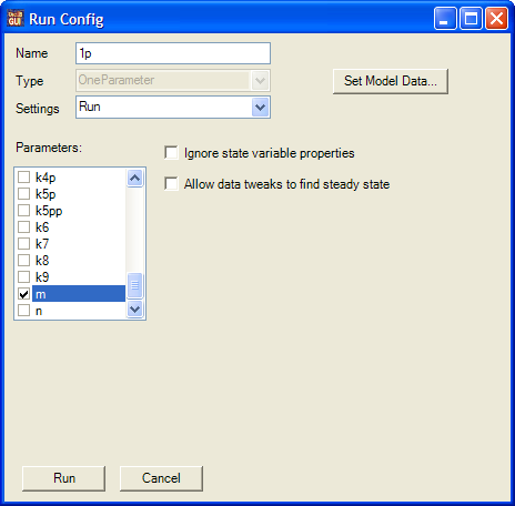

  

• Now, when you want to change some of the paramater values and/or state variables (collectively referred to in Oscill8 as the "Model Data"), you click on "Set Model Data..."; this opens the model data edit dialog. Notice that we have values, mins, maxs, and other data associated with each parameter and state varaible (state variables come at the top of the list). Scroll down to m, change the value to 0.1 and the max to 25; then click OK. Click Run in the run config to complete the run.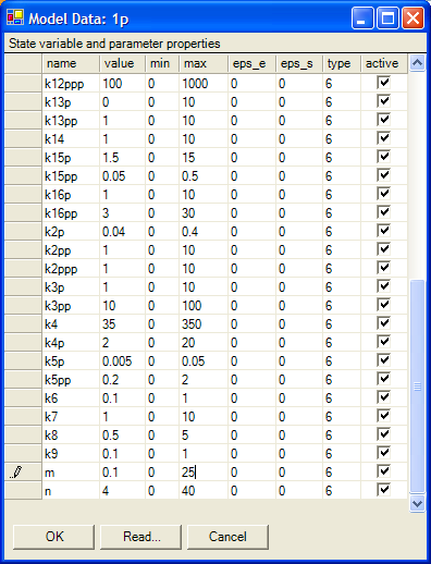

  

• The resulting graph will have a bunch of stuff crammed down into the lower left hand corner of the graph; use x and y to stretch the graph to the right and up. This still leaves a bit of a mess, so, let's choose a different state variable (that happens to be important for this model anyway). In the legend, toggle "CycBT" to on and "CKIT" to off; then alt-click to get the plot properties dialog and change the ranges to x: 0 to 2 and y: 0 to 1. This will give you: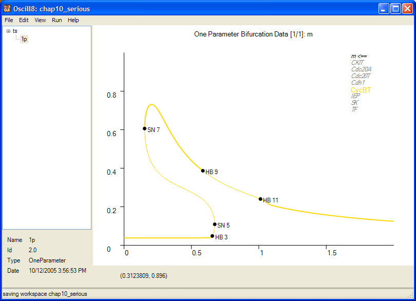

  

  Here, you can see a number of bifurcation points, including saddle-nodes (SN) and Hopf (HB) bifurcation points. By right clicking any of these, you'll see extra option on the context menu, including "Two Parameter" and "Follow Limit Cycle" (for HB only). Try "Follow Limit Cycle" by alt-clicking on HB 11; now we'll need to adjust a few settings to get a faster computation. Click the pulldown menu for "Settings:" and choose "Continuation". This gives you a list of paramters (that you may be familiar with from AUTO). Change DS=-0.05, DSMIN=0.001, DSMAX=0.5, NTST=20 EPSL=1e-6, EPSU=1e-6, EPSS=1e-4, then click Run (and be patient... this may take 15-20 seconds to run).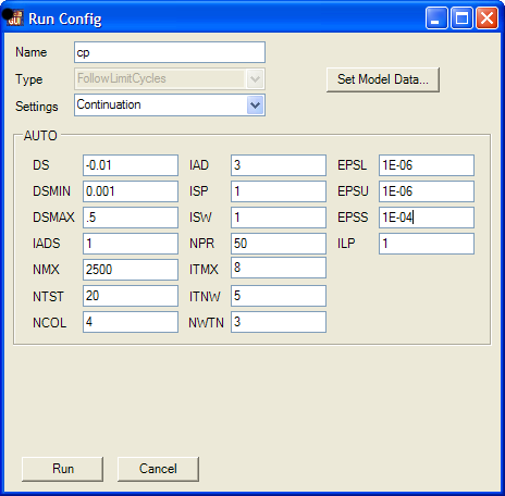

  

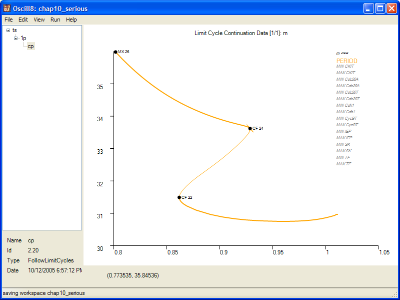
  As you can see, the default resulting plot is of the period of the limit cycle which branched off from the HB.

  

• Now, what we'd like to plot is the min/max of the oscillatory solution and combine it with the 1 parameter bifurcation diagram. We do this by toggling the period off, toggling MIN CycBT and MAX CycBT on, and clicking r to reset the plot. This gives you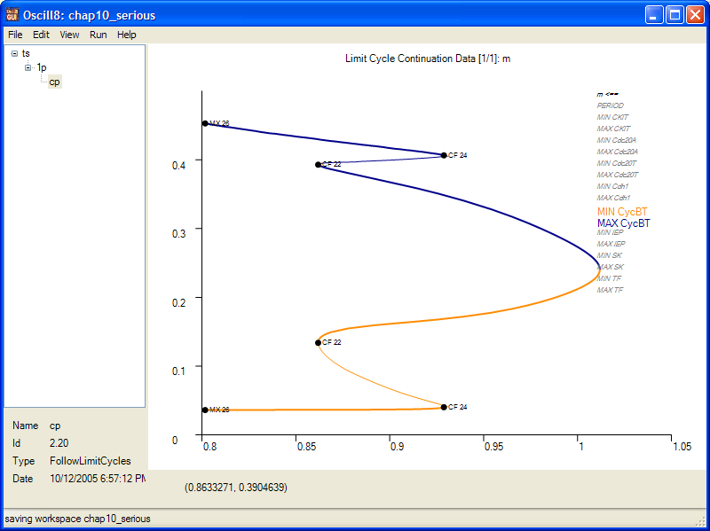

  

  Now, the fun part! Go back to our prepared one parameter diagram (by navigating in the history one node up, should be called "1p" unless you changed the name of it). If you see the one parameter diagram, then use the drag-and-drop graphics feature by grabbing the "cp" run just created (in the run history area, again) and drag it onto the graphic where you see the bifurcation values... COOOL! You should see:

  

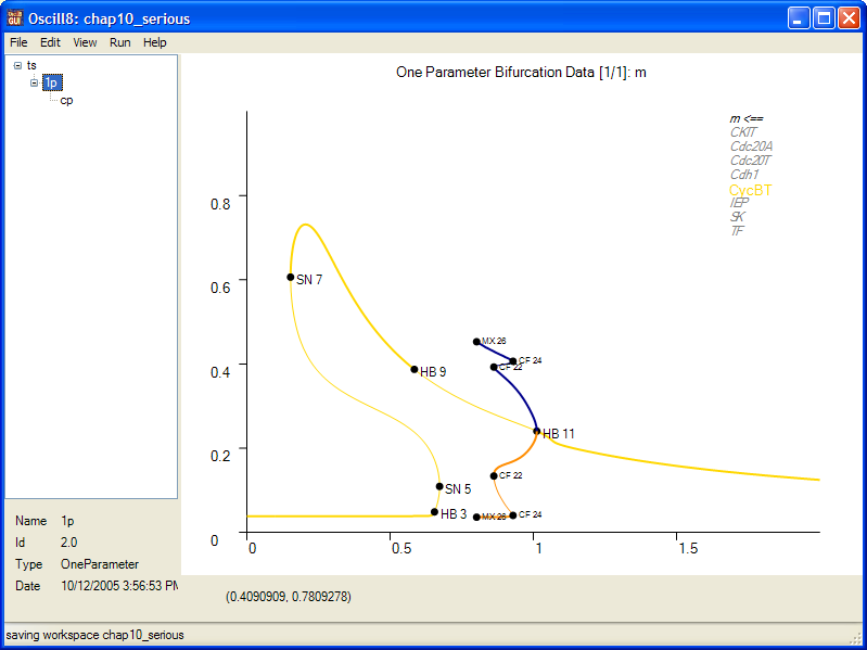
  Alternatively, you could have dragged the "1p" run onto the graphic of the "cp" run. In this case, you would see (after a double-click in the graphic and a shift-x control-shift-x to adjust the axes):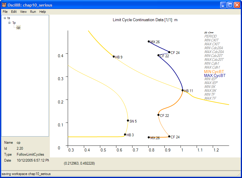

  

• We could've also choosen to continue any of the bifurcation points with respect to other parameters (a "Two Parameter" run). Do this for the parameter "k4" from HB 11, HB 3, and SN 5... playing with the color and width for the HB (red) and SN (green) loci, you might get something like this (after dragging and dropping and adjusting the axes):

  

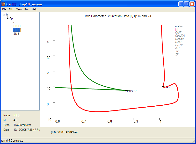
• Now, let's take a quick look at the RunSet, a collection of predefined runs that we can store and look at (and rerun) with some base set of parameter values. This run type is extremely useful for adjusting parameters to your liking. So, clicking back on the original "ts" run, let's alt-click --> Run --> RunSet. Alt-click in the "Run" area and select Add --> TimeSeries. Do the normal configure for the run and click Done. Again, alt-click in the "Runs" area and select Add --> One Parameter; set up a one parameter run (for the parameter m as before BUT in this case, you cannot adjust the parameters--we'll do that in a minute).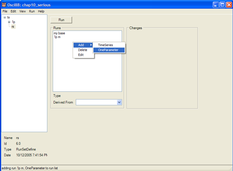

  

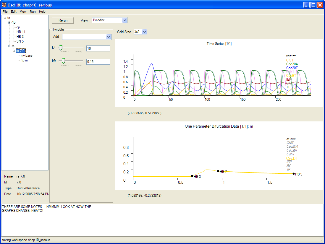
  Now, the area to the right labeled "Changes" allows us to make changes to the shared basal parameter set. So, for example, in the case of the one parameter run, we'll need to ensure that m is small since, in this particular case, the newton solver cannot locate a starting steady state given the default value of m (although in many cases it can--it just happens for this example, it doesn't--by design!). So we can alt-click in the "Changes" area (after highlighting the one parameter run in the "Runs" area), and add a change to m, set to 0.1. Now highlight both runs in the "Runs" area and click the Run button. There should be a new run, named "rs 6.0" or something; select it. You may need to increase your windows size for this, but do it; it's worth it! Now, from the "Grid Size" pulldown, select "2x1", voila! Double-click on the one parameter graphic and adjust it as above (toggle CKIT off, CycBT on, x=0 to 2, y=0 to 1). One last thing: from the "Add" dropdown menu in the "Twiddle" section (to the left), add "k4" and "k9", two of the system parameter we're going to twiddle. You should hopefully see something like: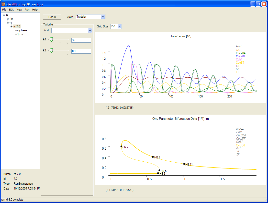

  

  Now, change k9 with the slider (or by typing in the box) to 0.15 and click rerun. Notice how the quality of the oscillation changed quite a bit and that the one paramter bifurcation diagram has morphed into a slight different shape. Then, change k4 to 20, 15, and then 10, notcing how the graphs change as rerun each time. You can watch as bifurcations disappear and the wave-form changes.

  

1. alt-clicking in the history area --> Notes --> View to add notes to any run you like
2. clicking on a graphic plot and pressing control-p to save the graphic to a bmp/png/jpg
3. alt-click in history area --> Print --> Summary to print a summary to the printer (or PDF, if you have that installed--here's a sample).